Python 株のSuperTrendのインジケーターを作成する

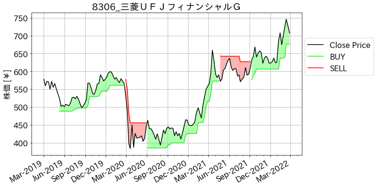
　本記事では、下図のようなスーパートレンドのIndicatorを作成する雛形コードを載せました。株の売買判定をする指標のひとつであるATR(Average True Range)を計算して、チャートに図示します。

　必要なのは、株価に関する時系列データで日付と高値、安値、終値です（下図）。

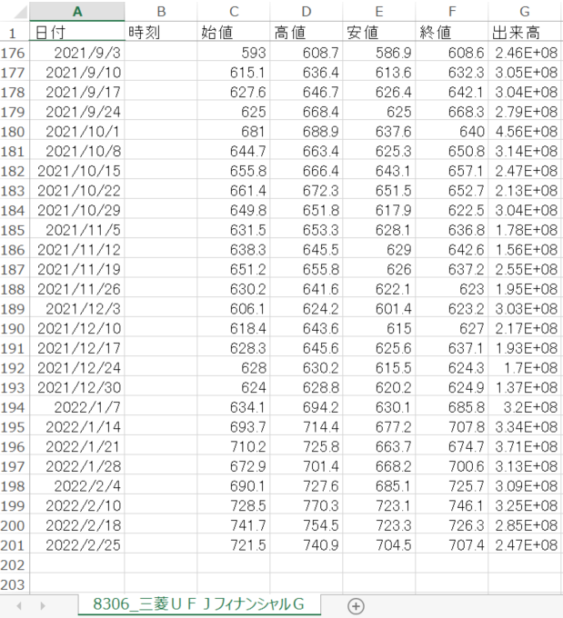
　ちなみに、上記のようなチャート情報は、証券会社に口座開設すれば、比較的容易に入手可能です。例えば、楽天証券の場合は下記リンク先を参考に入手できます。

hk29.hatenablog.jp

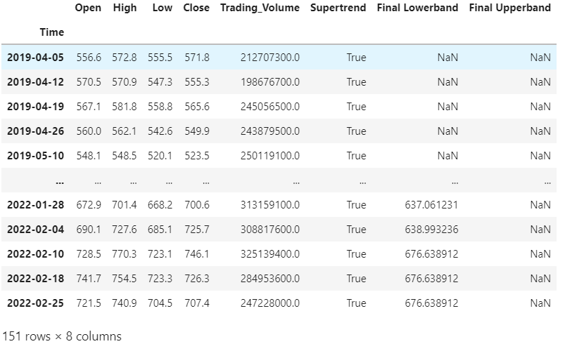
　本コードを実行すると、スーパートレンドとそれを図示するための計算を行い、下図のように列に追記します。

■本プログラム

#!/usr/bin/env python
# coding: utf-8

# In[1]:


import os
import pandas as pd
import numpy as np
import datetime
now = datetime.datetime.now()
#now = now.strftime("%y%m%d")

file_path = '8306_三菱ＵＦＪフィナンシャルＧ.csv'
file_name, _ = os.path.splitext(os.path.basename(file_path))
df1 = pd.read_csv(file_path)
print(file_name)
df1


# In[2]:


# 不要な列を削除する
df2 = df1.drop(['時刻'], axis=1)
df2


# In[3]:


# 列名を一括で変更する
target_column_list = ['日付', '始値', '高値', '安値', '終値', '出来高']
rename_column_list = ['Time', 'Open', 'High', 'Low', 'Close', 'Trading_Volume']
df3 = df2.rename(columns=dict(zip(target_column_list, rename_column_list)))
df3


# In[4]:


# 日付を時刻型へ変換
df3['Time'] = pd.to_datetime(df3['Time'])
df3


# In[5]:


# 現在から3年前のデータまでを対象にするため、時間の演算
from dateutil import relativedelta

# 秒, 時間,　日の場合
#my_time = now + datetime.timedelta(days = 3, hours = 5)
# 月, 年の場合は、dateutilのrelativedeltaを使う
my_time = now + relativedelta.relativedelta(years = -3)
print(my_time.year, my_time.month, my_time.day)


# In[6]:


# pandasの日付列に対して、特定の日時を指定しての区間抽出
DF = df3.copy()

# #DF = DF[DF['Time'] > datetime.datetime(2019, 1, 1)]
DF = DF[DF['Time'] >  datetime.datetime(my_time.year, my_time.month, my_time.day)]
DF.reset_index(drop = True, inplace = True)
DF


# In[7]:


# インデックスを列名で指定
DF.set_index('Time', inplace=True)
DF


# In[8]:


# ATR計算の係数
atr_period = 10
atr_multiplier = 2

high = DF['High']
low = DF['Low']
close = DF['Close']

# ATR(Average True Range)の計算
price_diffs = [high - low, 
               high - close.shift(), 
               close.shift() - low]
true_range = pd.concat(price_diffs, axis=1)
true_range = true_range.abs().max(axis=1)
atr = true_range.ewm(alpha = 1 / atr_period, min_periods = atr_period).mean() 

# 上下バンドの計算
final_upperband = upperband = (high + low) / 2 + (atr_multiplier * atr)
final_lowerband = lowerband = (high + low) / 2 - (atr_multiplier * atr)
print(final_upperband, final_lowerband)


# In[9]:


# スーパートレンドを図示するための処理
# 上ラインは赤色、下ラインは緑で表記。さらに色塗りするため

supertrend = [True] * len(DF) # 一旦、Trueで埋める
for i in range(1, len(DF.index)):
    curr, prev = i, i-1
    
    if close[curr] > final_upperband[prev]:
        supertrend[curr] = True
    elif close[curr] < final_lowerband[prev]:
        supertrend[curr] = False
    # その他の場合は、既存トレンドを継続する
    else:
        supertrend[curr] = supertrend[prev]
        if supertrend[curr] == True and final_lowerband[curr] < final_lowerband[prev]:
            final_lowerband[curr] = final_lowerband[prev]
        if supertrend[curr] == False and final_upperband[curr] > final_upperband[prev]:
            final_upperband[curr] = final_upperband[prev]
    
    # トレンドでない方の列には、欠損値nanを代入（その区間は、図示させないための処理） 
    if supertrend[curr] == True:
        final_upperband[curr] = np.nan
    else:
        final_lowerband[curr] = np.nan

# 作成したデータをpandasデータフレームで作成する。        
df_buf = pd.DataFrame({
    'Supertrend': supertrend,
    'Final Lowerband': final_lowerband,
    'Final Upperband': final_upperband
}, index=DF.index)
# 元のデータフレームへ追記する
DF = DF.join(df_buf)
DF


# In[10]:


# グラフ化
import matplotlib.pyplot as plt
from matplotlib import dates as mdates
import japanize_matplotlib
plt.rcParams['font.size'] = 16 # グラフの基本フォントサイズの設定

fig = plt.figure(figsize = (10, 6))
ax = fig.add_subplot(111)

plt.plot(DF.index, DF['Close'], c = 'k', label='Close Price')
plt.plot(DF.index, DF['Final Lowerband'], c = 'lime', label = 'BUY')
plt.plot(DF.index, DF['Final Upperband'], c = 'red', label = 'SELL')

# 塗り潰し
ax.fill_between(DF.index, DF['Close'], DF['Final Lowerband'], facecolor='lime', alpha=0.3)
ax.fill_between(DF.index, DF['Close'], DF['Final Upperband'], facecolor='red', alpha=0.3)

# 横軸を時間フォーマットにする
plt.gca().xaxis.set_major_formatter(mdates.DateFormatter('%b-%Y'))
plt.gca().xaxis.set_minor_locator(mdates.MonthLocator(interval = 1))
plt.gca().xaxis.set_major_locator(mdates.MonthLocator(interval = 3))
plt.gcf().autofmt_xdate()

plt.ylabel('株価 [￥]')
plt.title(file_name)
plt.legend(bbox_to_anchor = (1.28, 0.85))
plt.grid()
plt.show()


# In[ ]:

以上

<広告>

リンク

リンク